

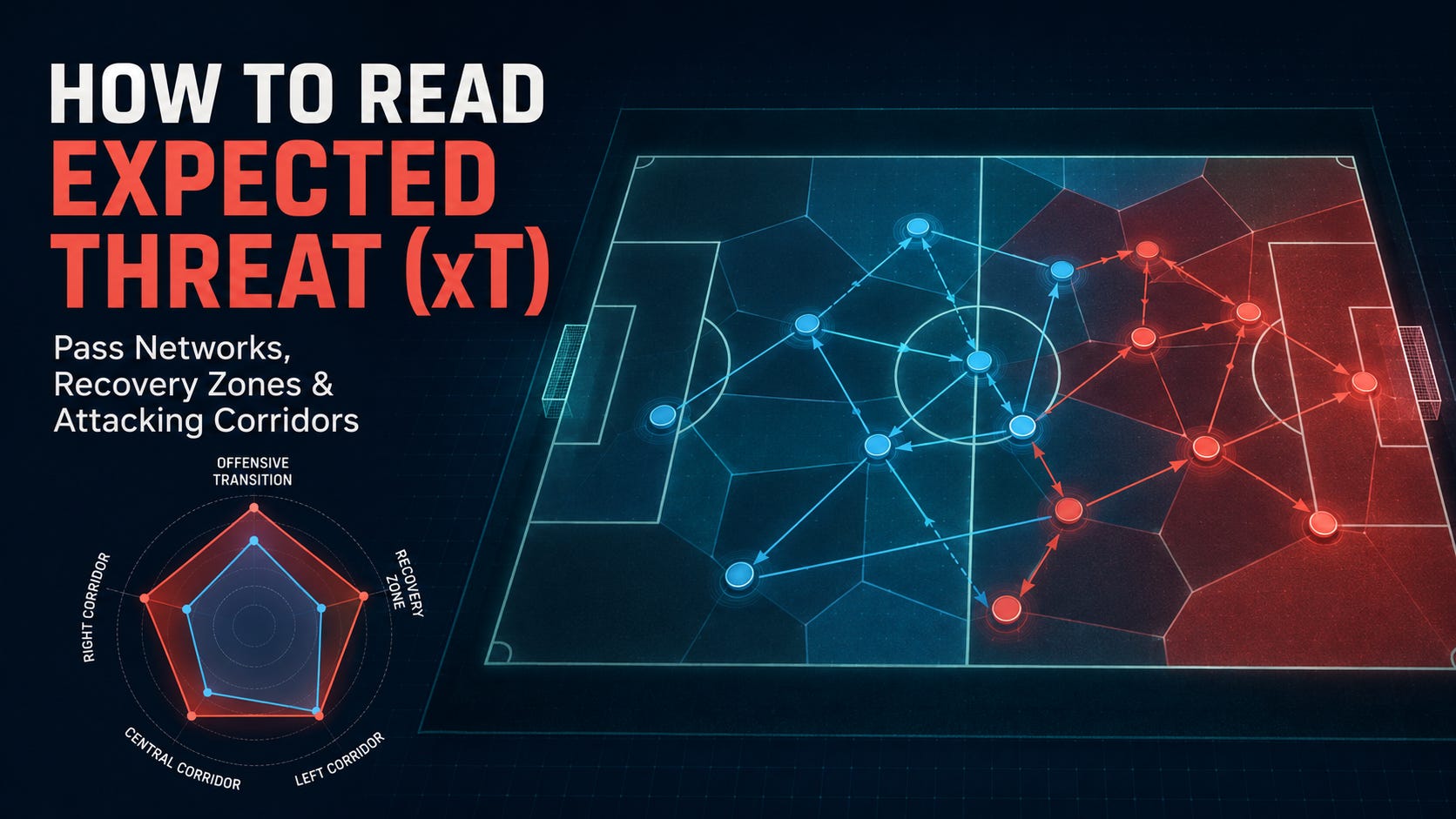
Football data becomes truly valuable when different visualizations begin to explain one another.
A pass network can show how a team circulates the ball. A Voronoi diagram can help us understand spatial influence. Expected Threat, commonly abbreviated as xT, estimates how much attacking danger is associated with moving the ball into a particular area of the pitch.
Individually, each tool provides part of the story. When interpreted together, however, they allow us to investigate a much more interesting question:
How does a team’s structure help it create, preserve or recover attacking threat?
This is the purpose of the xT metrics available in the Football Hacking web application. Instead of presenting xT as a single total, the platform separates it into tactical dimensions:
Offensive Transition xT
Recovery Zone xT
Left Corridor xT
Central Corridor xT
Right Corridor xT
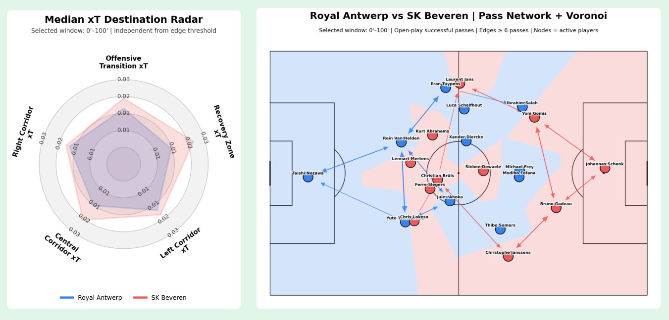
These metrics can then be interpreted alongside the pass network and the Voronoi map. The radar chart summarizes the team’s threat profile, while the network and spatial visualization help explain how that profile emerged.
This guide does not evaluate the specific match displayed in the reference image. Its purpose is to teach you how to interpret this type of football analytics visualization in any match.
If you want to explore the broader project and its data-driven approach to football analysis, visit Football Hacking.
What Is Expected Threat in Football?
Expected Threat is a possession-value model designed to estimate how much danger exists when the ball reaches a particular area of the pitch.
The basic logic is intuitive: receiving the ball close to the opponent’s penalty area is generally more threatening than receiving it next to your own corner flag. However, xT does more than simply reward proximity to goal. It considers how frequently possession from different zones leads to increasingly dangerous actions.
A successful action can increase threat when it moves the ball from a lower-value zone to a higher-value zone.
In simplified form:
xT added = value of the destination zone − value of the origin zone
Imagine that a player receives the ball in a zone with an xT value of 0.01 and completes a pass into a zone valued at 0.04. The action creates approximately 0.03 xT.
That does not mean there is now a literal 3% probability of scoring immediately. It means that, according to the model, the possession has moved into a substantially more threatening state.
This distinction matters because xT is not the same as expected goals.
Expected Goals, or xG, evaluates shots. Expected Threat evaluates how possession is moved toward situations from which dangerous attacks and shots may eventually emerge. In that sense, xT helps us study the construction of danger before the final attempt.
Why a Single Total xT Number Is Not Enough
A total xT value can tell you which team generated more cumulative threat, but it cannot fully explain how that threat was created.
Two teams may finish a match with similar xT totals while following completely different tactical paths.
One team may progress through patient combinations in the central corridor. Another may attack almost exclusively through wide areas. A third may struggle during settled possession but become dangerous immediately after recovering the ball.
If we only compare total xT, those differences disappear.
That is why the Football Hacking radar separates xT into tactical categories. The radar is not intended to replace the pass network. It acts as a compact summary that directs your attention toward the areas of the network that deserve closer inspection.
Think of the radar as the diagnosis and the network as the examination that helps explain it.
Understanding the Median xT Destination Radar
The radar shown in the Football Hacking interface is based on the xT associated with the destination of successful actions.
This is an important detail.
The visualization is not merely counting passes into a corridor. It is evaluating the typical threat value of the zones reached by those actions. A team can complete many passes on one side without producing a high corridor xT value if most of them end in harmless areas.
By using the median destination xT, the radar also reduces the influence of a small number of extreme actions.
Suppose a team completes twenty low-threat passes through the right corridor and one exceptionally dangerous pass into the penalty area. An average may be pulled upward by that single event. The median is more resistant to this distortion and gives us a better idea of the team’s typical attacking destination.
The radar should therefore be read as a representation of recurring territorial threat, not simply total passing volume.
A larger value on one axis means the team’s successful actions in that category generally reached more threatening destinations. It does not automatically mean that the team completed more actions, controlled more possession or created more shots.
Offensive Transition xT
Offensive Transition xT measures the threat generated during the first phase after the team regains possession.
In the Football Hacking methodology, offensive transitions are examined through short sequences following a recovery, with the initial progression limited to a defined number of passes. This isolates the moment in which the opponent may still be reorganizing defensively.
A high Offensive Transition xT value suggests that the team was regularly able to turn recoveries into forward-moving, threatening possessions.
This can happen through several mechanisms:
A direct vertical pass immediately after winning the ball
A ball recovery by a midfielder positioned between opposing lines
A wide player receiving before the defensive block can shift
A forward becoming available behind an advanced defensive line
A short combination that escapes counter-pressure
A carry or pass into a substantially more valuable zone
However, the radar alone cannot tell us which mechanism was responsible. This is where the pass network becomes essential.
How to Connect Offensive Transition xT to the Pass Network
When Offensive Transition xT is high, inspect the network for players who create a bridge between the recovery zone and the attacking structure.
Look for:
Long or strongly vertical connections
Central players connected to both defensive and attacking teammates
Wide outlets positioned beyond the opponent’s midfield line
Forwards with incoming connections from deeper players
Passing relationships that bypass several opponents
Players whose average positions make immediate progression possible
A team may have a high transition value without showing an extremely dense network. Fast attacks often depend on a limited number of highly valuable connections rather than long passing sequences.
Conversely, a dense network does not guarantee dangerous transitions. It may reflect secure circulation after the opponent has already recovered its defensive shape.
The key question is not “How many passes are visible?” It is:
Do the visible connections offer a plausible route from regaining possession to reaching a high-threat zone quickly?
Recovery Zone xT
Recovery Zone xT represents the threat value associated with the areas in which possession is regained.
Recovering the ball near the opponent’s penalty area is fundamentally different from recovering it deep inside your own defensive third. The first situation may place the team only one pass away from a shot. The second still requires the team to travel through several layers of pressure.
A high Recovery Zone xT value suggests that the team frequently regained possession in areas that already carried meaningful attacking potential.
This may indicate:
Effective high pressing
Successful counter-pressing after losing possession
Strong anticipation of the opponent’s passes
Control of second balls
Interceptions in advanced midfield positions
Defensive actions performed by forwards or attacking midfielders
Territorial dominance that trapped the opponent near its own goal
It is important not to interpret this metric as a complete measure of defensive quality. A team can defend very well in a low block and still have a modest Recovery Zone xT because its recoveries occur far from the opponent’s goal.
The metric answers a narrower and more tactical question:
How threatening was the territory in which the team recovered possession?
Reading Recovery Zones Through the Voronoi Map
The Voronoi layer divides the pitch according to which player is closest to each area. It provides a geometric approximation of spatial influence based on player positioning.
When Recovery Zone xT is high, use the Voronoi diagram to investigate whether the team’s structure supported advanced recoveries.
For example, look for:
Several players influencing space inside the opponent’s half
Small opposing territories near the ball
Midfielders positioned close enough to support pressure
Compact distances between attacking and midfield units
Coverage behind the first pressing line
Spatial control around likely passing destinations
A recovery does not happen in isolation. The player who wins the ball may receive the statistical credit, but the surrounding structure often makes the recovery possible.
One player presses the ball carrier. Another blocks the nearest passing option. A third covers the space behind them. The Voronoi diagram helps reveal this collective geometry.
If the team has high Recovery Zone xT but appears spatially stretched, the advanced recoveries may have resulted from isolated events, individual anticipation or opponent errors. If the high value is supported by compact and overlapping areas of influence, it may reflect a more repeatable pressing structure.
Left Corridor xT
Left Corridor xT measures the typical threat associated with successful actions whose destinations fall within the left attacking corridor.
A high value indicates that the team regularly reached dangerous zones on that side. It does not necessarily mean the left winger was solely responsible.
Left-side threat can be produced by:
An overlapping full-back
An inverted winger moving toward the half-space
A midfielder drifting wide
A striker pulling toward the channel
Diagonal switches from the opposite side
Combinations between three or more players
Repeated access to the area around the corner of the penalty box
To understand the metric, inspect the average positions and connections on that side of the network.
If the left-back, midfielder and winger form a clear triangle, the team may be progressing through combinations and positional support. If the left winger appears relatively isolated but receives strong diagonal connections, the threat may come from switches of play. If a central midfielder occupies the left half-space, the apparent wide threat may actually be generated from an inside position.
This is why corridor xT should not be reduced to the performance of the nominal winger.
Central Corridor xT
Central Corridor xT evaluates the threat associated with actions reaching central destinations.
Central progression is usually difficult because defending teams naturally protect the space in front of their goal. As a result, a high Central Corridor xT can reveal an important ability to play through or between defensive lines.
Possible tactical explanations include:
A midfielder receiving on the half-turn
A number ten finding space between the lines
A striker dropping to connect play
A third-man combination
A central overload
A line-breaking pass from a defender
A recovery that immediately creates a central attack
A winger moving inside and opening the outside lane
The pass network should be examined for central connectors. These are players whose positions and relationships link multiple units of the team.
A highly connected central player may act as a hub, but connection volume alone is insufficient. Many short sideways passes can produce a prominent network node without creating much threat.
Compare the player’s location, the direction of the edges and the Central Corridor xT value. If the team has a strong central network but low central threat, it may be circulating in front of the defensive block. If both the central network and central xT are strong, the structure is more likely to be breaking lines and reaching valuable areas.
Central xT and Spatial Occupation
The Voronoi map can add another layer of interpretation.
Look at how much central territory is controlled by the attacking team and whether the relevant players are positioned close enough to combine. Large areas of influence are not automatically positive. Sometimes a player controls a large polygon precisely because teammates and opponents are far away.
What matters is the tactical context.
A central player surrounded by nearby passing options may support rapid combinations. A central player isolated inside a large territory may technically influence space but still lack a safe route for receiving or releasing the ball.
Use the pass network to identify relationships and the Voronoi layer to judge spatial conditions around those relationships.
Right Corridor xT
Right Corridor xT follows the same logic as the left-side metric, but it evaluates destinations in the right attacking corridor.
The most useful analysis usually comes from comparing both sides.
A strong asymmetry may reveal:
A deliberate attacking preference
The influence of a particularly creative player
An advanced full-back on one side
An inverted winger on the other
A weak point in the opponent’s defensive structure
Difficulty progressing through one corridor
A buildup structure designed to attract pressure before switching play
Match-state effects that changed the direction of attacks
Asymmetry is not necessarily a weakness. Many successful teams attack unevenly by design.
One side may be responsible for progression while the other provides width. One full-back may advance aggressively while the opposite full-back remains deeper to protect defensive balance. One winger may receive to feet, while the other attacks space behind the defense.
The radar tells you that the destinations differed in threat. The network helps you determine whether that difference came from player roles, positioning or passing relationships.
How the Radar and Pass Network Explain Each Other
The most reliable workflow is to move back and forth between the two visualizations rather than reading either one independently.
Step 1: Identify the Strongest xT Dimension
Begin with the radar and determine which axis extends furthest.
Is the team’s strongest characteristic offensive transition, recovery location, central progression or one of the wide corridors?
Do not immediately explain why. At this stage, you are only identifying the pattern.
Step 2: Compare the Teams’ Profiles
Look at the shape of both polygons.
One team may have a balanced profile, with similar values across all corridors. Another may show a pronounced peak in a specific dimension. Similar overall sizes can hide very different tactical identities.
Ask:
Is one team more transition-oriented?
Does one team recover possession in more threatening areas?
Is one side clearly preferred?
Is central progression a major point of difference?
Is the profile balanced or specialized?
Step 3: Locate the Relevant Players in the Network
Once you identify the strongest or weakest radar axis, move to the corresponding area of the pass network.
For a high Left Corridor xT, inspect the left-sided players and their connections. For a high Central Corridor xT, examine central hubs and line-breaking links. For a high Offensive Transition xT, search for direct routes connecting deeper recoveries to advanced receivers.
Step 4: Use the Voronoi Layer to Examine Space
Now study the surrounding territories.
Did the team create numerical or spatial advantages around the important connections? Were key receivers positioned in zones where they could influence large areas? Was the opponent’s structure fragmented? Did the attacking team occupy the corridor with one player or several complementary players?
The Voronoi map is particularly useful for understanding why a passing relationship may have been available.
Step 5: Check Whether the Explanation Is Structurally Plausible
Avoid inventing a tactical story from a single number.
Your explanation should be supported by multiple elements:
The radar identifies the type of threat
The pass network identifies the relationships
Average positions identify the team’s structure
The Voronoi map provides spatial context
Edge direction helps reveal the movement of possession
Edge thresholds distinguish repeated connections from occasional ones
When these pieces point in the same direction, the interpretation becomes stronger.
Why Edge Thresholds Matter
In a pass network, edges usually represent successful passing relationships between players. To prevent the visualization from becoming unreadable, a minimum threshold may be applied.
For example, an edge may only appear when a passing connection occurred at least a certain number of times during the selected window.
This means an absent line does not necessarily prove that two players never exchanged a pass. It may simply mean that their connection did not reach the visualization threshold.
This distinction is especially important when interpreting xT.
A rare pass can create substantial threat, but it may not appear as a visible network edge if the connection occurred only once or twice. Meanwhile, a thick or prominent edge may represent frequent circulation without high destination xT.
The network emphasizes repeatability. The xT radar emphasizes destination quality. Reading them together prevents you from confusing frequency with danger.
The Importance of the Selected Time Window
Football structures change throughout a match.
A team may begin with aggressive pressing, retreat after scoring, change shape after a substitution or attack more directly during the final minutes. A full-match visualization can combine all these phases into one average structure.
The selected time window therefore matters enormously.
When analyzing a defined interval, make sure both visualizations refer to the same period. Otherwise, you may compare an xT profile from one phase of the match with a pass network representing another.
Useful windows include:
The opening 15 minutes
The period before the first goal
The period after a tactical change
The minutes played with a specific lineup
A phase of sustained pressure
The final 20 minutes
Equal-score and losing-game states
The period before and after a red card
Smaller windows provide tactical specificity but also contain fewer actions. Larger windows provide more data but may blur important changes.
There is no universally perfect interval. The correct window depends on the question you want to answer.
Common Mistakes When Interpreting xT Visualizations
Treating xT as a Goal Prediction
xT measures the value of ball progression into threatening areas. It does not guarantee a shot, a goal or even a successful final action.
A team can accumulate promising possession value and still make poor decisions near the penalty area.
Assuming More Possession Means More Threat
Possession can be sterile. A team may dominate the ball through safe defensive circulation while its opponent produces more dangerous progression from fewer actions.
Confusing Passing Volume With Passing Value
A heavily used connection is not automatically a valuable connection. Always compare the network with the xT profile.
Treating Corridor xT as a Winger Rating
Corridor threat is a collective outcome. Full-backs, midfielders, forwards and players switching the ball can all contribute to the same side.
Ignoring Match Context
Scoreline, substitutions, red cards, fatigue and tactical instructions can alter both structure and threat generation.
Reading Voronoi Polygons as Permanent Control
A Voronoi map is a spatial approximation based on player locations. It does not directly account for body orientation, acceleration, pressing intensity or the time required to reach the ball.
It should support tactical interpretation, not replace it.
Drawing Conclusions From Tiny Differences
Small differences between radar values may not represent a meaningful tactical gap. Focus first on clear patterns, consistent asymmetries and relationships supported by the network.
A Practical Example Without Evaluating a Specific Match
Imagine that Team A has a high Right Corridor xT but a modest Central Corridor xT.
On the network, its right-back, right midfielder and right winger form a dense triangle. The right winger receives several progressive connections, while the central attacking midfielder remains deeper and has few links with the striker.
The Voronoi map shows that Team A controls useful space on the right, with the winger influencing the outside lane and the midfielder occupying the adjacent half-space.
A reasonable interpretation would be that Team A’s structure successfully creates threat through right-sided combinations but has greater difficulty accessing central zones between the opponent’s midfield and defensive lines.
Now imagine that Team B has a higher Offensive Transition xT and Recovery Zone xT, but a less dense pass network.
Its structure may be less focused on long possession sequences. Instead, advanced recoveries and direct connections may allow it to reach dangerous destinations with fewer passes.
Neither style is automatically superior. The visualizations reveal how each team creates threat, not whether one tactical identity is universally better.
From Description to Tactical Explanation
The real value of football analytics lies in moving beyond statements such as:
“Team A attacked more on the right.”
A deeper explanation would be:
“Team A consistently reached higher-threat destinations through the right corridor. Its pass network shows repeated connections among the right-sided full-back, midfielder and winger, while the spatial map suggests that these players maintained complementary areas of influence. The combination of corridor xT, network structure and territorial occupation indicates that the right side was not merely active—it was the team’s most reliable mechanism for advancing possession into dangerous areas.”
That is the difference between describing a visualization and interpreting it.
The goal is not to use complex metrics to make football sound complicated. The goal is to use the metrics to make hidden tactical relationships easier to see.
Final Thoughts
Expected Threat becomes far more informative when it is separated into tactical categories and connected to the structure behind the actions.
Offensive Transition xT helps us understand how effectively a team transforms recoveries into danger. Recovery Zone xT shows whether possession is being regained in threatening territory. Left, central and right corridor xT reveal where successful progression reaches its most valuable destinations.
The pass network then identifies the players and relationships responsible for moving the ball. The Voronoi layer adds spatial context by showing how influence is distributed around those relationships.
The radar tells you where the threat appears. The network helps explain who connects the structure. The Voronoi map suggests how the surrounding space supports or restricts those connections.
Used together, these tools provide a more complete picture of football tactics than possession percentages, pass totals or isolated event counts can offer.
Explore the methodology, visual analysis tools and the wider project at Football Hacking, where football structure is examined through data without separating numbers from the tactical context that gives them meaning.